Time-Series Storage Inside Postgres, Without a Chunk Catalog
SnoutTime is a time-series extension for Postgres that we built for SnoutData Cloud. It keeps Postgres's own partitioning as its only partition catalog, rewrites closed partitions into a column store, and keeps rollups current from partial states that merge. This is the first of two reports: the design, measured against the Postgres it is built on, at 10 and 100 million rows. The second compares it with the other time-series extensions for Postgres, adds a billion rows, and goes to their authors for comment before it is published.
Why build one
Time-series data in Postgres is usually served by an extension that partitions by time, compresses closed data column by column, and maintains aggregates incrementally. The most widely used one licenses its compression and incremental aggregates so that they cannot be offered as a hosted database, and a hosted database is what SnoutData Cloud is. So we built SnoutTime from scratch, without reading that extension's source, to do the same jobs inside every Cloud project. Its source is on GitHub, snoutdata/snouttime, under the Apache License 2.0.
Four questions shaped the design, and each has a measurement below:
- Is Postgres's declarative partitioning enough to manage time-series tables without a catalog of our own?
- What does sealing only closed partitions into a column store cost, and what does it buy?
- Do mergeable partial states make a rollup refresh cost what changed, and no more?
- Is an as-of join done as one merge faster than the SQL form, and when is it not?
Every result comes with its history: the first time it was measured, what that showed was wrong, and what changed. Most of the design's speed was not in its first version. The first sealed partitions answered "the last reading of every host" in 11.5 seconds at 10 million rows on our development laptop; the same query takes 7.5 ms there now, and each step between the two was found by measuring. The losses are told the same way.
The design
A series table is a partitioned table
A series table is a Postgres partitioned table plus one catalog row. SnoutTime makes partitions ahead of the data, seals them, drops them for retention and moves existing data into them, but it keeps no partition catalog of its own. Pruning, pg_dump, logical replication and every tool that understands partitions keep working unchanged, because the partitions are Postgres's. Converting an existing table moves no data at first: the table becomes the new table's default partition, so converting a billion rows takes as long as converting none, and rows move into real partitions one partition at a time afterwards.
Closed partitions become a column store
The partition being written stays an ordinary Postgres table, so an insert is a plain Postgres insert with no SnoutTime code on its path. Once a partition's time has passed, it is sealed: rewritten into SnoutTime's table access method, sorted by a key (host, then time, in the benchmark). It is the column store of C-Store [2], confined to time ranges that are closed, so the write path stays Postgres's own. A sealed partition stores row groups of 8,192 rows, each column encoded by its type (delta-of-delta and bit-packing for times and integers, XOR with the previous value for floats, after Gorilla [1]; dictionaries and runs for repetitive text) and then compressed. Integer and float columns are split into pages of 1,024 rows, each compressed and checksummed on its own, so a narrow read decodes only the pages its rows are in.
Each partition keeps a small directory: every row group's first and last key, and where each host's rows end inside it. That makes a sealed partition its own index on its key. Finding a host is a binary search over the directory, and the partition needs no separate index for it, which is most of why it is small. The store is written once per seal through Postgres's bulk-write path, so it is logged, replicated and restored like an index build.
Late rows are never refused
A row that arrives for a sealed partition goes to a small ordinary table beside it, and a delete goes to a delete log. Both are plain Postgres tables, so transactions and visibility are Postgres's own. A read merges them in; a reseal folds them back in once they pass a tenth of the partition.
Reading a sealed partition
Four read paths, each chosen by the planner on cost beside Postgres's own, and each held by the tests to exactly the answer Postgres gives without it: a column scan that reads only the columns a query uses and skips row groups by their minima and maxima; an aggregate node that does the first half of Postgres's two-phase aggregation on encoded columns, a row group at a time; a last-point node that finds each host's latest row from the directory without decoding; and a row that decodes a column only when the executor asks for it.
One more piece is about planning, not reading. Postgres will not prune partitions by ts >= '…' - interval '1 hour' while planning, because adding a day or a month depends on the session's time zone. An hour does not, so SnoutTime computes that sum while planning; for days and months it adds a bound that holds in every time zone (a month is 28 to 31 days, a day 24 local hours, and no two zones differ by more than 26 hours), and keeps the original comparison beside it.
Rollups and the as-of join
A rollup is an ordinary table of per-bucket partial states. A write records the time range it touched, and a refresh recomputes only those buckets. Every aggregate a rollup may hold can be merged (sums, counts, minima, maxima, first and last values, and sketches whose states combine: t-digest [5] for percentiles, HyperLogLog [6, 7] for distinct counts), which is what lets a refresh touch one bucket without its neighbours [3, 4]. The as-of join finds, for each event, the latest reading at or before its time for the same key; SnoutTime does it as one merge of the two sides in time order, where plain SQL does one index probe per event.
How we measured
- The machine: an EC2 m7gd.4xlarge (Graviton3, 16 vCPUs, 64 GiB, local NVMe), Debian 13, nothing else running. Anyone can rent the same one. The run was split across three identical machines, each comparison kept on one of them; plain Postgres ran on two, and they agreed within 1.3% on every query but one (4.2%).
- The version: SnoutTime 0.1.4, the one SnoutData Cloud runs.
- The targets: fresh containers from the same Postgres 17.11 image, each limited to 4 CPUs and 8 GB, with the same settings and the same indexes. Plain Postgres as one table and as a table partitioned by day, and SnoutTime with every partition sealed.
- The data: a CPU-monitoring workload of ten metrics per reading, a reading every 10 seconds from 100 hosts (10 million rows) or 1,000 hosts (100 million), and an IoT shape with 2,500 devices, jitter, gaps and late rows. Both generators are plain SQL and deterministic.
- The queries: six, chosen before the design was built: the last reading of every host, per-host and fleet aggregates over a day and a week, a selective filter, an as-of join and a top ten. The same SQL on every target.
- Timing: one warm-up and five timed runs, the median reported, every run kept in the record.
Size and ingest
| 10M rows | 100M rows | |
|---|---|---|
| Plain partitioned Postgres | 1.91 GB | 21.27 GB |
| Sealed SnoutTime | 0.70 GB (0.37x) | 7.04 GB (0.33x) |
| Sealing, after the load | 13.5 s | 193 s |
| Load speed, as a share of Postgres's | 100.0% | 100.7% |
With partitions made ahead, SnoutTime is not on the insert path at all, so the load shows it adds nothing, not that it is faster. On the IoT shape the sealed table is 100 MB against Postgres's 936 MB.
Query times
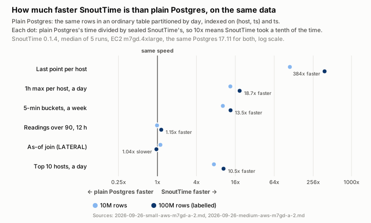
| Median ms, Postgres / SnoutTime | 10M rows | 100M rows |
|---|---|---|
| Last reading of every host | 2,189 / 19.6 (112x) | 61,464 / 160 (384x) |
| 1h max per host over a day | 292 / 21.8 (13.4x) | 3,074 / 165 (18.7x) |
| 5-minute buckets over a week | 700 / 68.1 (10.3x) | 8,349 / 619 (13.5x) |
| Readings over 90 in 12 hours | 19.3 / 19.6 (0.99x) | 160 / 140 (1.15x) |
| As-of join (LATERAL) | 202 / 181 (1.11x) | 2,083 / 2,160 (0.96x) |
| Top 10 hosts over a day | 139 / 18.6 (7.5x) | 1,387 / 132 (10.5x) |
- The last reading of every host is not a fair fight, and it says why sealing matters most. The query is
DISTINCT ON (host) ... ORDER BY host, ts DESC, the same on every target, and Postgres 17 has no index skip scan, so plain Postgres reads every row. Someone tuning Postgres would rewrite it to skip from host to host through the index and get a very different number. We run the same SQL everywhere, so the 384x is what the same SQL costs, not what an expert could make Postgres do. - Aggregates over a day or a week are 10 to 19 times faster: the aggregate node reads two or three of the table's twelve columns, a row group at a time.
- The as-of join is level at 100 million rows (1.04x slower) and 1.11x faster at 10 million. Plain Postgres as a single table, not partitioned, is the fastest of all on it at 100 million (1,949 ms).
The result that went backwards
One number got worse between versions, and publishing it is what found why. The as-of join, on the same machine type:
| Version | 10M rows | 100M rows | Against Postgres at 100M |
|---|---|---|---|
| 0.1.1 | 223 ms | 3,706 ms | 1.8x slower |
| 0.1.3 | 209 ms | 5,670 ms | 2.7x slower |
| 0.1.4 | 181 ms | 2,160 ms | 1.04x slower |
At 10 million rows, with 100 hosts, it had improved, so the regression only showed at 1,000 hosts. We reproduced it on a laptop with 1,000 hosts and the same stored bytes timed under each version, bisected it to the change that made late-row lookups fast, measured two guesses that turned out wrong, and then profiled it. To keep its cache of decoded row groups within work_mem, a scan added up the size of every cached group each time it loaded one. With 100 hosts the cache holds a handful; with 1,000, an as-of join keeps hundreds, and each of 205,590 probes walked them all. Each cached group now keeps its own size, and the scan the total.
How it got fast
The first sealed partitions were slower than the plain tables they replaced on every query but one. On the development laptop at 10 million rows (history, not a result: that machine shares itself with everything else):
| Query | First sealed | Later | What moved it |
|---|---|---|---|
| Last reading of every host | 11,500 ms | 7.5 ms | A node that reads only the key and time columns; checksums on the CPU's CRC instruction, which had cost three times the decoding; the directory recording where each host's rows end; pages of 1,024 rows read on their own |
| 1h max per host, a day | 130 ms | 11.6 ms | Aggregates on the encoded columns, a row group at a time; the checksum |
| Readings over 90, 12 hours | 101 ms | 10.2 ms | The filter applied before a row is formed, and row groups skipped by filters like now() - interval, which until then had never skipped one |
| Top 10 hosts, a day | 123 ms | 10.3 ms | The aggregate node and the checksum |
Late rows, rollups and the as-of join
Late rows. In one sealed partition of 10 million rows, the last 10 readings of one host take 0.40 ms clean, 0.40 ms with 1% of the rows late and 1% deleted, and 0.55 ms at 10%. That lookup once took 95 ms at 1% and 1,138 ms at 10%, until it read only that host's late rows through an index and read deletes per row group. Scans pay more: 1.4 to 2.1 times at 1% and 3.4 to 11 times at 10%, which is why a reseal folds late rows back in once they pass a tenth of the partition.
Sealing without blocking readers. Rewriting a partition in place holds readers for the whole rewrite, 4.6 seconds at 10 million rows. SnoutTime builds the column store beside it and swaps it in, which holds a reader for 0.26 seconds and takes 1.9 times as long in total.
Rollups. Hourly per host over 100 million readings (278,000 buckets), a full recompute takes 39.5 seconds; after one late row the refresh takes 0.54 seconds, 72 times less, and reading the rollup takes 75 ms against 10.6 seconds for the same aggregate over the raw table. The honest half: invalidation is by time range, so 100 late rows in 100 different hours cost 13.4 seconds, a third of a full recompute.
The as-of join as a merge. With as many events as readings (10 million), snouttime.asof_join takes 15.3 seconds against 89.2 for LATERAL, 5.8 times faster, and 1.8 times with a tenth as many. With 20,000 events it is 18 times slower, because the merge reads the whole right side where LATERAL does 20,000 index probes. Choosing between the two by the sizes is not built yet.
A second data shape. On the IoT data (2,500 devices, three days, jitter, gaps, late rows): the last reading of every device 97.8 ms against 9,106, one device hourly 1.10 against 4.94, the fleet in 15-minute buckets over six hours 60.9 against 128.
What is not done
- Two data shapes, both generated. A real workload compresses the way it compresses.
- One machine type so far, and one load per target. A billion rows is the second report.
- The six queries were chosen by us, before the design was built.
- A filter bounded by
now() - intervalstill plans every partition; bounds are computed while planning for constants only. - Aggregates over whole chunks are 4 to 6% slower than two versions ago at 100 million rows, the cost of decoding by page, which is what made the narrow reads fast.
What this comparison is, and is not
- The same Postgres, settings, limits, indexes and SQL on every target. Plain partitioned Postgres is what SnoutTime is built on, so the difference between the two is what sealing and the read paths add.
- The SQL is not tuned per target. Postgres would answer the last reading of every host far faster with a hand-written query that skips from host to host through its index. We wrote no such query for any target.
- Plain Postgres is not a time-series system, and beating it on time-series queries is what an extension like this is for. Where SnoutTime stands among the other time-series extensions is the second report.
- Where SnoutTime is slower, it is in the tables, not left out.
We did our best to make these comparisons fair. If you think we got one wrong, write to [email protected] and we will re-run it and publish the correction.
References
- T. Pelkonen, S. Franklin, J. Teller, P. Cavallaro, Q. Huang, J. Meza, K. Veeraraghavan. "Gorilla: A Fast, Scalable, In-Memory Time Series Database." PVLDB 8(12), 2015.
- M. Stonebraker et al. "C-Store: A Column-oriented DBMS." VLDB 2005.
- J. Gray et al. "Data Cube: A Relational Aggregation Operator Generalizing Group-By, Cross-Tab, and Sub-Totals." Data Mining and Knowledge Discovery 1(1), 1997.
- P. K. Agarwal, G. Cormode, Z. Huang, J. M. Phillips, Z. Wei, K. Yi. "Mergeable Summaries." PODS 2012.
- T. Dunning, O. Ertl. "Computing Extremely Accurate Quantiles Using t-Digests." 2019.
- P. Flajolet, É. Fusy, O. Gandouet, F. Meunier. "HyperLogLog: the analysis of a near-optimal cardinality estimation algorithm." AofA 2007.
- S. Heule, M. Nunkesser, A. Hall. "HyperLogLog in Practice." EDBT 2013.
SnoutTime runs in every SnoutData Cloud project, and its source is at github.com/snoutdata/snouttime. Every number here comes from a recorded run that keeps the image, the command and every timed run beside the median. The second report, the comparison with the other time-series extensions for Postgres, follows.